Peiyuan Pang received his master’s degree from the South China University of Technology in 2021. He is currently a doctoral candidate at the Institute of Applied Physics and Materials Engineering, University of Macau. His research mainly focuses on perovskite electroluminescent devices
Guichuan Xing received his Ph.D. degree in Physics from the National University of Singapore in 2011. He is currently a Professor at the Institute of Applied Physics and Materials Engineering, University of Macau. His major research interests include ultrafast laser spectroscopy, nano optoelectronics, and perovskite for light harvesting and light emission
Metal halide perovskites, as a promising semiconductor material, have been successfully used in electroluminescent devices because of their desirable characteristics, such as good conductivity, high color purity, tunable bandgap, low cost and solution process ability. In the past few years, significant progress has been made in the development of high-efficiency perovskite light-emitting diodes (PeLEDs). These efficient PeLEDs are mainly achieved by sophisticated spin-coating methods, which can easily control the perovskite's composition, film thickness, morphology and crystallinity. However, with the continuous development of PeLEDs, commercial production problems have to be solved, such as large area production, high resolution patterning and substrate diversity, which are difficult for the current spin-coating process.
Graphical Abstract
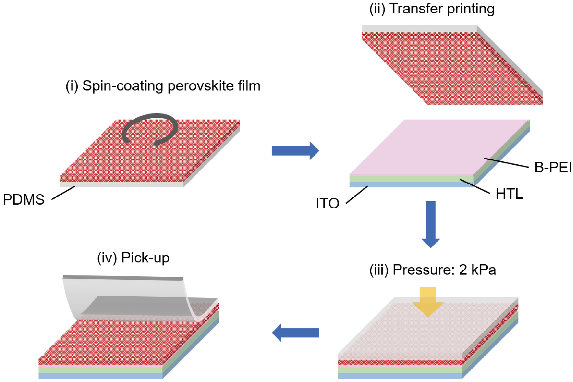
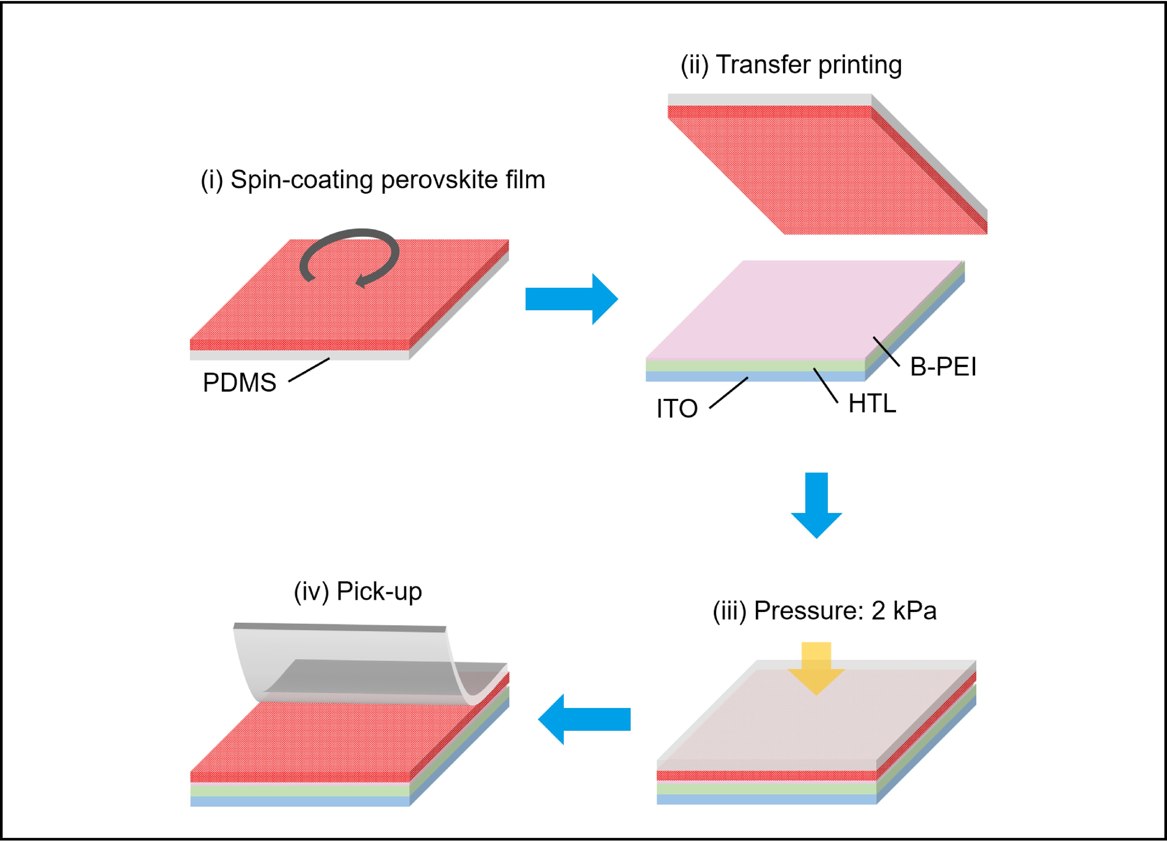
Schematic illustration of the modified transfer printing process.
Abstract
Metal halide perovskites, as a promising semiconductor material, have been successfully used in electroluminescent devices because of their desirable characteristics, such as good conductivity, high color purity, tunable bandgap, low cost and solution process ability. In the past few years, significant progress has been made in the development of high-efficiency perovskite light-emitting diodes (PeLEDs). These efficient PeLEDs are mainly achieved by sophisticated spin-coating methods, which can easily control the perovskite's composition, film thickness, morphology and crystallinity. However, with the continuous development of PeLEDs, commercial production problems have to be solved, such as large area production, high resolution patterning and substrate diversity, which are difficult for the current spin-coating process.
Public Summary
This research highlight summarizes a robust mass transfer printing method for perovskite films fabrication with nanostructures reported by Xiao and colleagues.
This transfer printing method enables the fabrication of large-area perovskite nanostructures with high resolution.
Using this method, white PeLEDs with red and sky-blue emission perovskite micro-stripes has been achieved.
High-power laser interactions with plasma have been widely studied since the 1970s. Most of these studies and applications are related to energy and momentum coupling from laser to plasma. Applications include particle accelerators[1], X-ray sources, inertial confinement fusion, etc. Plasma waves are an important collective effect driven by high-power laser pulses. Energy and momentum are proven to be exchanged with high efficiency between charged particles and the field (laser or plasma field) in this process, which are the foundations of many applications. For example, the self-generated magnetic field plays an important role in laser-plasma interactions. The inverse Faraday (IF) effect for circularly polarized (CP) light[2–5] is one of the well-known methods of laser-driven direct current magnetic field generation. This can be explained as the result of spin angular momentum (SAM) transfer from light to plasma. For a CP light beam, every photon has a SAM of ℏ. Here, σ=±1 are for the right and left circular polarizations. On the other hand, light can also possess orbital angular momentum (OAM)[6] and thereby have the potential to create plasmas with OAM. The OAM of a photon is due to the helical wavefront instead of the circular polarization. Mathematically, we can use a basis set of orthogonal Laguerre-Gaussian (LG) modes to express any helical wavefronts. For one pure LG mode with a twist index of l, every photon has lℏ of OAM. While such twisted light in conventional optics at low intensities has been widely studied (e.g., light tweezers[7]), high-intensity (I>1016 W/cm2) twisted light has received moderate attention very recently. Unavoidably, the interaction medium will be plasma. Various new simulation phenomena and theories on interactions between intense LG mode laser beams and plasma have been proposed[8–22]. In experiments, several works have been reported[16, 23–28]. However, high-efficiency OAM exchange between the plasma and field still needs more attention.
In previous work[29], electron plasma waves with a helical rotating structure and static, axial magnetic field generation were confirmed using three-dimensional particle-in-cell (PIC) simulations. Now, we will give a general theory and more details under the condition of paraxial approximation where the spot size of the laser beam is large enough. The ponderomotive force of beating OAM lasers will be analyzed first. Then, the electrons will be driven to oscillate in a way to generate a twisted electron density. The associated axial magnetic field will be calculated using general theory and compared with the simulation results. Studies on the damping of twisted plasma waves and the axial magnetic field have been published in Refs. [21, 30, 31]. This paper is organized as follows: in Section 2, we demonstrate the ponderomotive potential for two beating LG laser pulses and one LG laser pulse. Both of them are different from the ponderomotive potential of a Gaussian pulse. In Section 3, we show the electric field, the helical electron density, and the magnetic field generation of twisted plasma waves in simulations. In Section 4, we give a general theory of twisted plasma waves driven by the beating of two LG beams. The helical electron density and the magnetic field are accurately described in theory. In Section 5, we explore the scheme of using the beating of an LG beam and a Gaussian beam.
2.
The twisted ponderomotive potential using two beating LG-CP laser pulses
It is convenient to write down a Laguerre-Gaussian (LG) transverse electromagnetic field with polarisation vector ^es in cylindrical coordinates (r,θ,x) as
with the eigenfunction Fp,l(X) given as Fp,l(X)=Cp,lX|l|/2e−X/2Llp(X) where the normalized radial co-ordinate X=2r2/w2(x) is specified, Llp(X) is a Laguerre polynomial with Cpl=√2p!/[π(p+|l|)!] (C01=√2/π≃0.8) being a normalisation to ensure an orthonormal set, the gouy phase ϕp,l=(2p+l+1)arctan(x/xR) and front surface curvature f(x)=x+x2R/x, the beam width wb(x)=wb,0√1+x2/x2R and wb,0=wb(0), the Rayleigh range is xR=kw2b,0. For the following analysis, we simplify it by only considering the region within the Rayleigh range so that terms with f(x) and ϕp,l can be ignored and we consider wb(x)=wb,0. Now we have an electric field from the laser as E=^es∑p,lEp,lFp,l(X)exp(ikx−iωt+ilθ).
In the context of the discussions about the OAM of light, the multiplier term of exp(−ilθ) in Eq. (1) is the most significant one. It sets the twist of the wavefronts and determines the OAM of a mode. The OAM per photon for this mode is lℏ, where l is the twist index. The laser pulse can efficiently exchange OAM with a structured target upon reflection[8], but the same cannot be said about a helical pulse propagating through a uniform plasma. This can be illustrated by examining the direction of the ponderomotive force induced by a helical beam with electric field amplitude E and frequency ω on plasma electrons,
Fpond=−∇Φpond,Φpond=e24meω2|E(r,t)|2,
(2)
where Φpond is the ponderomotive potential and e and me are the electron charge and mass, respectively. The intensity of |E|2 is independent of θ and it follows from Eq. (2) that Φpond has no dependence on θ (see Fig. 1a). Therefore, the ponderomotive force Fpond of a single LG beam has only a radial component in the cross section of the beam and it induces no azimuthal rotation of the plasma. The ponderomotive force is nonlinear, so the discussed difficulty can be overcome by using two co-propagating LG modes with different frequencies and twist indices to generate a ponderomotive force with a substantial azimuthal component.
Figure
1.
Structure of the ponderomotive potential Φpond (in a. u.) of one LG laser pulse (a) and two beating LG laser pulses (b) in transverse plane (y-z). The ponderomotive force Fpond=−∇Φpond has an azimuthal component only for two beating waves.
We illustrate this for a pair of LG waves that have p=0 and opposite twist indices, l1=−l2=l, so that they have the same radial dependence. The waves are beating with slightly different frequencies: ω1=ω0 and ω2=ω0−Δω, where Δω≪ω0. We keep the radial normalization equivalent for all modes such that the real part of the final electric field looks like:
E=^esE0Fp,l(X)[cos(k1x−ω1t−lθ)+cos(k2x−ω2t+lθ)].
(3)
Considering an average over the timescale tfast=2π/(ω1+ω2) and length scale xfast=2π/(k1+k2), we have a slowly varying electric field of the form:
Eslow=^es2E0Fp,l(X)cos(−Δkx2+Δωt2+lθ),
(4)
where Δk=k1−k2. This slowly varying envelope of the total electric field retains all of the angular momentum of the two combined waves. It is worth mentioning that the wave travels in the same direction as the sum of its parts, despite the sign change in k. To find the ponderomotive force we use the relation:
Putting a0=eE0/(meω0c), the ponderomotive potential can be described as
Φpond=0.5mec2a20F2p,l(X)(1+cos(−Δkx+Δωt+2lθ)).
(6)
The ponderomotive potential is then no longer cylindrically symmetric (see Fig. 1b). The resulting ponderomotive force, Fpond=−∇Φpond, has an azimuthal component and slowly rotates in the cross section of the propagating beams, i.e., in the y-z plane. In contrast, Fpond produced by a superposition of conventional beams without OAM (l=0) has no azimuthal component. The remainder of this work will elucidate twisted plasma waves driven by the twisted ponderomotive force and axial magnetic field generation related to the axial OAM carried by electrons.
3.
Simulation results driven by twisted ponderomotive force
Using EPOCH[32], we performed three-dimensional PIC simulations on the interactions between two beating LG-CP beams and plasma. For two LG-CP beams (p=0), we choose the l+σ=0 to get zero angular momentum. Therefore, magnetic field generation due to the IF effect is excluded. Some key simulation parameters are summarized in Table 1. The two LG-CP beams have frequencies and twist indices of ω1=ω0, ω2=0.9ω0 and l1 = –1, l2 = +1, respectively. The frequency difference is set as the same as the plasma frequency ωp=0.1ω0. ωp=√4πn0e2/me is the plasma frequency, where n0 is the electron density and ω0 is the frequency of beam 1 with a wavelength of 0.8 μm. The target is initially set as a fully ionized hydrogen plasma with uniform density n0=4.5×1018 cm−3 and zero temperature. Both the incident pulses have a Gaussian shape with a total duration of τg =200 fs and a beam width of wb=10 μm, and the electric field amplitude of Ey, z = 1.0 TV/m. For the beam 1, the corresponding peak dimensionless vector potential of a0=0.25.
Table
1.
3D PIC simulation parameters. nc=1.8×1021 cm−3 is the critical density corresponding to the laser wavelength 0.8 μm.
In the following, we will give the main simulation results. The twisted electric field (Er, Eθ, Ex) distributions are shown in Fig. 2. We should note that the non-zero distribution of Eθ (see Fig. 2b) clearly shows twist characteristics, which do not exist in normal longitudinal plasma waves. Furthermore, we find that the phase distributions of Er (see Fig. 2a) and Ex (see Fig. 2c) are twisted with azimuth θ. These are different compared to longitudinal plasma waves driven by the beating of two Gaussian beams where there would be no dependence on θ[33]. Of particular note are the twisted electron density perturbations δne presented in Fig. 3a and a static axial magnetic field Bx in the y-z plane, shown in Fig. 3c. The magnetic field can be as high as 8 T and persists for hundreds of femtoseconds after the laser beams pass by. We also observe an azimuthal magnetic field distribution which is presented in Fig. 3e. The dashed lines on the right of Fig. 3 are line-outs from the slices plotted against the position along the line-outs d plotted in the left of Fig. 3. As time passes, the twisted electron density rotates around the x-axis with angular frequency ωpe. The scheme works for other choices of different twist indices (see 3D PIC simulation results in Section 5). There, twist effects using an LG and a Gaussian beam are confirmed and likely to be easier to realize experimentally. However, to simplify the theoretical analysis, we choose opposite twist indices in the following analysis. We also choose circularly polarized lasers instead of linearly polarized lasers to exclude the effects of polarization deflection due to the twisted electron density. The dependence of the polarization deflection on the laser frequency can lead to a symmetry break in the transverse plane. Frequency detuning effects should be discussed for a real experiment. Additional simulations have been accomplished with different beating frequencies. We found that the axial magnetic fields are in similar distributions although a weaker peak amplitude (≈90%) when the beating frequency is Δω=(1.00±0.05)ωp.
Figure
2.
3D PIC simulation results of electric field and fluid velocity distribution at transverse plane (y-z plane) at the centre of simulation box (x = 15 μm) and the time 320 fs after the laser has passed by. (a), (b), and (c) show transverse slices of Ex, Eθ, and Er.
Figure
3.
PIC results of transverse profile of (a) electron density perturbation δne, (c) axial magnetic field Bx and (e) azimuthal magnetic field Bθ at the centre of simulation box (x = 15 μm) and the time 320 fs after the laser has passed by. The dashed lines shown in the transverse slices are the line outs used to plot the graphics on the right. The plots on the right, (b), (d), and (f), are line outs from the slices plotted against the position along the line outs d plotted in (a), (c), and (e). d is the coordinate along the dashed lines. Solid lines in (b), (d) and (f) are theory predictions, for the same situation considered in Table 1.
4.
The general theory of twisted plasma waves driven by twisted ponderomotive force
First, we solve the non-relativistic cold electron-fluid equations driven by the twisted ponderomotive force in Section 2. Using linear fluid theory (LFT)[32], we can describe laser-driven electron plasma waves as
{me∂tu=e∇Φ+Fpond∂tδne+n0∇⋅u=0∇2Φ=4πeδne.
(7)
Here, ions are assumed to be immobile, and δne is the difference between the electron density ne and ion density n0. u is the velocity of the electron fluid and Φ is the static electric potential. The resulting equation for the perturbations of electron density δne in a plasma with an initially uniform electron density n0 has the form
∂2tδne+ω2peδne=n0me∇Fpond.
(8)
This equation is analogous to the equation that describes a driven harmonic oscillator. The driving item can be calculated as
\begin{split} \nabla^2\Phi_\text{pond}=& \dfrac{a_0^2}{2} F^2_{p,l}(X)\left[-\Delta k^2-\dfrac{8 l^2}{Xw_b^2} + \dfrac{8}{w_b^2}G_{p,l}(X)\right]\cdot\\ &\cos\left(-\Delta k x +\Delta\omega t +2l\theta\right) + \dfrac{4a_0^2}{w_{\rm{b}}^2} F^2_{p,l}(X)G_{p,l}(X). \end{split}
(10)
We will only consider the part with the cosine which will drive our forced plasma oscillation. When the ponderomotive force drives the perturbations with a frequency equal to \Delta \omega = \omega_{\rm{pe}},we have a solution of \delta n_{\rm{e}} as
\begin{eqnarray} \dfrac{\delta n_{\rm{e}}}{n_0} &= \dfrac{\tau {\rm{c}}^2\Delta k^2a_0^2}{4\omega_{\rm{p}}} \Xi_{p,l}(X)\sin\left(-\Delta k x +\omega_{\rm{pe}} t +2 l\theta\right), \\ \Xi_{p,l}(X) &= F^2_{p,l}(X)\left[1+\dfrac{1}{\Delta k^2w_{\rm{b}}^2}\dfrac{8 l^2}{X} - \dfrac{8}{\Delta k^2w_{\rm{b}}^2}G_{p,l}(X)\right]. \end{eqnarray}
(11)
It suggests a linearly growing amplitude with the laser pulse duration \tau . Our simulation use two LG-CP beams having same parameters except different wavelengths and twist indexes ( p = 0, l_1 = - l_2 = l ).The function of \Xi_{p,l}(X) electron density perturbation can be presented in the following explicit form,
It is the same result as the Eq. (2) in Ref. [28]. If 1/\Delta k^2 w_{\rm{b}}^2 is small then \Xi_{p,l}(X) = F^2_{p,l}(X) for simple cases, and for cases where p=0 then \Xi_{0,l}(X) = C_{0l}X^{|l|}{\rm{e}}^{-X}/|l|!, this can calculate a situation for a Gaussian wave where l=0 so that \Xi_{0,0}(X)={\rm{e}}^{-X}. In this paper, we will focus on the case of paraxial approximation with small 1/\Delta k^2 w_{\rm{b}}^2.
In a similar way, the electric field {\boldsymbol{E}} and the velocity field {\boldsymbol{u}} can be solved in the following equations:
\begin{eqnarray} \left\{ \begin{array}{lr} F_{\text{pond},\theta} = (l {\rm{c}}^2 a_0^2m_{\rm{e}}/w_{\rm{b}})\sqrt{2/X} F^2_{p,l}(X)\sin\left(-\Delta k x +\Delta\omega t +2 l\theta\right)\\ F_{\text{pond},r} = -({\rm{c}}^2 a_0^2m_{\rm{e}}/w_{\rm{b}})\sqrt{2X}(F^2_{p,l}(X))'\cos\left(-\Delta k x +\Delta\omega t +2 l\theta\right) \\ F_{\text{pond},x} = -0.5({\rm{c}}^2 a_0^2m_{\rm{e}}\Delta k) F^2_{p,l}(X)\sin\left(-\Delta k x +\Delta\omega t +2 l\theta\right) \end{array}. \right. \end{eqnarray}
(14)
We can ignore the last part of the constant force in the radial direction. For the velocity we can again neglect the constant radial term giving {\rm{\partial}}_t F as,
\begin{eqnarray} \left\{ \begin{array}{lr} {\rm{\partial}}_tF_{\text{pond},\theta} = (l {\rm{c}}^2 a_0^2m_{\rm{e}}\omega_{{\rm{pe}}}/w_{\rm{b}})\sqrt{2/X} F^2_{p,l}(X)\cos\left(-\Delta k x +\Delta\omega t +2 l\theta\right)\\ {\rm{\partial}}_tF_{\text{pond},r} = ({\rm{c}}^2a_0^2m_{\rm{e}}\omega_{{\rm{pe}}}/w_{\rm{b}})\sqrt{2X}(F^2_{p,l}(X))'\sin\left(-\Delta k x +\Delta\omega t +2 l\theta\right)\\ {\rm{\partial}}_t F_{\text{pond},x} = -0.5({\rm{c}}^2a_0^2m_{\rm{e}}\omega_{{\rm{pe}}}\Delta k) F^2_{p,l}(X)\cos\left(-\Delta k x +\Delta\omega t +2 l\theta\right) \end{array}. \right. \end{eqnarray}
(15)
Mirroring the approach used above, the electric field and fluid velocity are found to be
\begin{eqnarray} \left\{ \begin{array}{lr} E_{\theta} = -0.5\tau\omega_{{\rm{pe}}} l {\rm{c}}^2 a_0^2(m_{\rm{e}}/e/w_{\rm{b}})\sqrt{2/X} F^2_{p,l}(X)\cdot\\ \qquad \cos\left(-\Delta k x +\Delta\omega t +2 l\theta\right)\\ E_{r} = -\tau\omega_{{\rm{pe}}}({\rm{c}}^2 a_0^2m_{\rm{e}}/e/w_{\rm{b}})\sqrt{X/2}(F^2_{p,l}(X))'\sin\left(-\Delta k x +\Delta\omega t + 2 l\theta\right) \\ E_{x} = 0.25\tau\omega_{{\rm{pe}}}{\rm{c}}^2 a_0^2(m_{\rm{e}}/e)\Delta k F^2_{p,l}(X)\cos\left(-\Delta k x +\Delta\omega t +2 l\theta\right) \end{array} , \right. \end{eqnarray}
(16)
and
\begin{eqnarray} \left\{ \begin{array}{lr} u_{\theta} = -0.5(l {\rm{c}}^2 a_0^2\tau/w_{\rm{b}}) \sqrt{2/X} F^2_{p,l}(X)\sin\left(-\Delta k x +\Delta\omega t +2 l\theta\right)\\ u_{r} = ({\rm{c}}^2 a_0^2\tau/w_{\rm{b}})\sqrt{X/2}(F^2_{p,l}(X))'\cos\left(-\Delta k x +\Delta\omega t +2 l\theta\right)\\ u_{x} = 0.25({\rm{c}}^2a_0^2\tau\Delta k) F^2_{p,l}(X)\sin\left(-\Delta k x +\Delta\omega t +2 l\theta\right) \end{array}. \right. \end{eqnarray}
(17)
Using the explicit form of (F^2_{0, l}(X))' = (|l|/X - 1)F^2_{0, l} , we can get the same result as Eq. (s7) and Eq. (s8) in the supplemental material of Ref. [29].
In the theory above, the electric current density is {\boldsymbol j}^e = -e n_0 {\boldsymbol u}, and the displacement current density is {\boldsymbol j}^\text{dis} = {\rm{\partial}} {\boldsymbol E}/(4{\rm{\pi}} {\rm{\partial}} t). According to high-order fluid theory[34,35], the second-order current can generate a magnetic field even though {\boldsymbol j}^e + {\boldsymbol j}^\text{dis} = 0 in the first order. In the PIC simulation results, the time-averaged net current in both the azimuthal directions \langle j^{(2)}_{\theta} \rangle (i.e., net rotating current) and the axial direction \langle j^{(2)}_{x} \rangle are confirmed. With a definition of \widetilde{j_0}= -en_0\tau^2 c^4\Delta k^3a_0^4/\omega_{\rm{p}}, the second-order current is
\begin{eqnarray} \left\{ \begin{array}{lr} j^{(2)}_{\theta} = -(l/8) \widetilde{j_0}/(w_{\rm{b}}\Delta k) \sqrt{2/X} F^4_{p,l}(X)\sin^2\left(-\Delta k x +\Delta\omega t +2 l\theta\right)\\ j^{(2)}_{r} = (1/8)\widetilde{j_0}/(w_{\rm{b}}\Delta k)\sqrt{X/2}(F^2_{p,l}(X))'F^2_{p,l}(X)\cdot\\ \qquad \sin2\left(-\Delta k x +\Delta\omega t +2 l\theta\right)\\ j^{(2)}_{x} = (1/16)\widetilde{j_0} F^4_{p,l}(X)\sin^2\left(-\Delta k x +\Delta\omega t +2 l\theta\right) \end{array}. \right. \end{eqnarray}
(18)
The equation for the second-order vector potential {\boldsymbol{A}}^{(2)} can be written as
In the paraxial approximation where only the dominant axial derivative in the Laplacian term is accounted for, we can obtain the explicit expressions for the vector potential {\boldsymbol{A}}^{(2)} as
\begin{eqnarray} \left\{ \begin{array}{lr} A^{(2)}_{\theta} = -(l{\rm{\pi c}}/4) \widetilde{j_0}/(w_{\rm{b}}\Delta k) \sqrt{2/X} F^4_{p,l}(X)[\dfrac{1}{\Delta\omega^2} -\dfrac{1}{4\Delta k^2{\rm{c}}^2 - 3\Delta\omega^2} \cos2\left(-\Delta k x +\Delta\omega t +2 l\theta\right)]\\ A^{(2)}_{r} = ({\rm{\pi c}}/2)\widetilde{j_0}/(w_{\rm{b}}\Delta k)\sqrt{X/2}(F^2_{p,l}(X))'F^2_{p,l}(X)\dfrac{1}{4\Delta k^2{\rm{c}}^2 - 3\Delta\omega^2}\sin2\left(-\Delta k x +\Delta\omega t +2 l\theta\right)\\ A^{(2)}_{x} = (\pi {\rm{c}}/8)\widetilde{j_0} F^4_{p,l}(X)[\dfrac{1}{\Delta\omega^2} -\dfrac{1}{4\Delta k^2{\rm{c}}^2 - 3\Delta\omega^2} \cos2\left(-\Delta k x +\Delta\omega t +2 l\theta\right)] \end{array}. \right. \end{eqnarray}
(20)
The axial and azimuthal components contain a constant term and a second harmonic oscillating term. However, the radial component has only a second harmonic oscillating term. The quasi-stationary magnetic field can be calculated by {\boldsymbol{B}} = \nabla \times {\boldsymbol{A}}^{(2)},
The relationship between the azimuthal and axial components is B_{\theta}/B_{x} = 0.25(w_{\rm{b}}\Delta k/l)\sqrt{X}. With the parameters of \kappa_{{w}} = \Delta k w_{\rm{b}} and \kappa_n = \tau {\rm{c}}^2\Delta k^2a_0^2/(4\omega_{\rm{p}}), we can get the amplitude of B_x ,
If we have \kappa_w = 10 , \kappa_n = 0.1 and \widetilde{n_0} = n_0 / n_c , we can get B_{x0} (T) \sim 5 l \sqrt{\widetilde{n_0}} . It means that if we assume that the electron density perturbation is small and the paraxial approximation works well, the amplitude of B_x will increase with a larger plasma density. Since the plasma density cannot be overdense in our scheme here, we expect that there is an upper limit on the amplitude of B_x .
In the PIC simulation shown in Table 1, Fig. 2 and Fig. 3 give the results. Here, 1/w_{\rm{b}}^2\Delta k^2 = 0.016 when we use \Delta k = \omega_{{\rm{pe}}}/{\rm{c}}. For simplicity, Eq. (11) has been obtained assuming a flat-top pulse with duration \tau . For the truncated Gaussian pulse used in the PIC simulation (i.e., I(t) = 0 for |t - t_{\rm{p}}| \ge \tau_{\rm{g}}/2 where t_{\rm{p}}= \tau_{\rm{g}}/2 is the time of peak intensity), \tau =0.75\tau_{\rm{g}} is appropriate. The Eq. (16) shows that the radial field E_r is phase different compared to the azimuthal field E_{\theta} and axial fields E_{x} . These are the same as the results in Fig. 2. The radial field u_r is also phase different compared to the azimuthal field u_{\theta} and axial fields u_{x} according to Eq. (17). Both u_{\theta} \propto l and E_{\theta} \propto l show the importance of the OAM of the driving lasers. The calculation results of electron density perturbation in the transverse plane are shown as a solid line in Fig. 3b, which is close to the simulation result (dashed line). The difference is thought to be caused by ignoring the last part of the constant force in the radial direction in Eq. (10). Theoretical predictions of the magnetic field from Eq. (21) are shown as solid lines in Fig. 3d and f. They are also close to the dashed lines. The result of the LFT is twisted plasma waves with a helical rotating structure. It is different from the longitudinal plasma waves driven by the beating of two Gaussian lasers, where transverse profiles depend only on radius[33]. The magnetic field generation due to the second-order current is explained well in the paraxial approximation. While this study is limited to plasma waves with small amplitudes, the high-order terms are ignored in Eq. (7). In other simulations, we observed spiral phenomena that may be related to the high-order nonlinear terms.
To understand more details on the twisted plasma waves with electrons carrying axial OAM, we analyze the oscillating phase of a single electron under a transverse electric field of E_r = E_{r1}\sin \Phi_0 and E_{\theta} = E_{\theta 1} \cos \Phi_0 , where \Phi_0 = \omega_{\rm{p}} t + 2l\theta_0 at x = 0 and \theta_0 is the azimuth. Here, E_r(r_0, \theta_0) and E_{\theta}(r_0, \theta_0) are rewritten for our purpose according to Eq. (16). The solutions of the motion equation m_{\rm{e}} {\rm{d}}^2 {\bf r}_1/{\rm{d}}t^2 = -e{\boldsymbol E}(t, {\boldsymbol r}_0) to the first order in coordinates of (y, z) are
Within such an oscillating electric field, electrons will oscillate locally with an azimuthally dependent phase to the first order. The central shift velocity is assumed to be small and should have no contribution to the rotating phase \phi . If the amplitude dependence on the radius is kept only for positive and negative values, the dependence of the rotating phase \phi on azimuth \theta_0 is
where r_{\rm{b}} = w_{\rm{b}}\sqrt{(|l|/2)} and l = −1. Furthermore, we can show that the rotating electron density in the transverse plane comes from particles oscillating elliptically in the transverse plane with an azimuthally dependent phase. We reconstruct the 2D electron density perturbation in the transverse plane to a higher-order approximation from particle oscillation. This oscillation can be viewed as a mapping of the \mathit{\boldsymbol{r}}_0 space onto the \mathit{\boldsymbol{r}}_0 + \mathit{\boldsymbol{r}}_1 space. Here, we have \mathit{\boldsymbol{r}}_1 = \int (v_{y1}, v_{z1}) {\rm{d}}t. The mapping is assumed to be single-valued and regular here. Then, the number density due to the motion can be given by n{\rm{d}}V = n_0{\rm{d}}V_0, where the two volume elements ({\rm{d}}V_0 and {\rm{d}}V) are related by the Jacobian of the transformation[36]. From the electron oscillation, we can get
Here, we get v_{r1} = eE_{r1}/(m_{\rm{e}}\omega_{\rm{p}}) and v_{\theta1} = -eE_{\theta1}/(m_{\rm{e}}\omega_{\rm{p}}) from Eq. (23). The explicit form of Eq. (26) shows that the first order electron density is the same as the LFT result of Eq. (11) in the transverse plane if we ignore k_{\rm{p}} x. We can obtain the electric field in the azimuth component to a second order, E_{\theta} = E_{\theta 1}\cos \Phi_0 + o(\eta^2, r_0)\sin 2\Phi_0. To the first order, it is just the same as the electric field from LFT. We can write a demo with some randomly distributed particles rotating with a phase dependence of azimuth in the plane. The collected motion of rotation with a phase dependence of azimuth will create a rotating electron density and carry axial OAM. Such a rotating electron density in plasma will produce a twisted electrostatic field, which in reality can push every electron rotating with a phase dependence of azimuth. It is a self-consistency process in twisted plasma waves.
Finally, using the equation of \langle L_x^{\rm{e}} \rangle = -\langle j^{(2)}_{\theta} \rangle r m_{\rm{e}} /e, we can get the theoretical result of the transverse profile of the time-averaged axial OAM density. The integration of \langle L_x^{\rm{e}} \rangle over radius r is not zero when l \ne 0 . For electromagnetic fields, the energy and momentum of electromagnetic waves are transported essentially by electric and magnetic fields. But for the plasma wave fields, electrostatic waves in plasma carry energy but no momentum if we do not consider the magnetic field due to the high order effect. Only particles will carry axial momentum and OAM. The same results can also be found in Ref. [31]. In Refs. [30,31], Langmuir plasma waves carrying a finite OAM are studied using kinetic theory in the paraxial approximation. The dispersion relation and energy and momentum exchange between particles and the field in the damping process are studied for twisted plasma waves.
5.
Simulation results driven by beating between an LG pulse and a Gaussian pulse
Considering the difficulties of producing high intensity LG beams in experiments, we accomplished a simulation using the beating of one LG beam ( l = −1) and one Gaussian beam ( l = 0). Now, the ponderomotive force is {\boldsymbol F}_\text{pond}(r, \theta, x, t) \propto \nabla \cos(\omega_{\rm{p}} t - k_{\rm{p}}x - \theta) and then the electron density perturbation is \delta n_{\rm{e}} \propto \sin(\omega_{\rm{p}} t - k_{\rm{p}}x - \theta). We set the beam 2 in Table 1 as a Gaussian beam and the other parameters are kept the same. Their frequency shift was also set to match the plasma frequency. Similar twisted electron density and magnetic field generation are observed in Fig. 4. Of particular note are the single helical electron density distribution \delta n_{\rm{e}} presented in Fig. 4a. In Fig. 4b, the magnetic field can be as high as 20 T. In future experiments, we may consider using temporally-chirped pulses for twisted plasma wave excitation[37]
Figure
4.
PIC results of transverse profile of (a) electron density perturbation \delta n_e , (b) axial magnetic field B_x and (c) azimuthal magnetic field B_{\theta} at the centre of simulation box ( x = 15 μm) and the time 320 fs after the laser has passed by.
In conclusion, twisted plasma waves carrying OAM are produced in PIC simulations by using beating of two LG beams or one LG and one Gaussian beam. We compare the ponderomotive force of two beating LG beams with the ponderomotive force of two beating Gaussian beams. The substantial azimuthal component of the ponderomotive force provides a unique tool for an effective exchange of OAM between the light and the plasma. Twisted electron plasma waves with a rotating helical structure are confirmed using three-dimensional PIC simulations. Once being excited, the twisted plasma wave can persist in the plasma long after the laser beams that create the ponderomotive force are gone. Essentially, the electrons are left oscillating along elliptical orbits in the transverse plane with an azimuthally dependent phase offset. This collectively yields a persistent, rotating wave structure, and an associated with it nonlinear electron current. The current configuration that is similar to that in a solenoid creates a longitudinal quasi-static magnetic field. Under the condition of paraxial approximation, we develop a general theory to explain the twist of the plasma waves and calculate the distributions of the magnetic fields in axial and azimuthal directions. Finally, to relax the experimental conditions of getting relativistic twisted laser intensities, we run simulations using beating between an LG and a Gaussian beam. The twisted ponderomotive force and twisted plasma waves would be easier to realize experimentally when only one beam with OAM is needed.
Data availability
The datasets generated and analyzed during the current study are available from the corresponding author on reasonable request.
Code availability
PIC simulations were performed with the fully relativistic open-access 3D PIC code EPOCH[38].
Acknowledgements
This work was supported by USTC Research Funds of the Double First-Class Initiative (YD2140002003), Strategic Priority Research Program of CAS (XDA25010200), CAS Project for Young Scientists in Basic Research (YSBR060), and Newton International Fellows Alumni follow-on funding. Simulations were performed with EPOCH (developed under UK EPSRC Grants EP/G054950/1, EP/G056803/1, EP/G055165/1, and EP/M022463/1). The Computational Center of USTC and Hefei Advanced Computing Center are acknowledged for computational support.
Conflict of interest
The authors declare that they have no conflict of interest.
Preprint statement
Research presented in this work was posted on a preprint server prior to publication in JUSTC. The corresponding preprint article can be found here: arXiv: 2211.01630. https://arxiv.org/abs/2211.01630.
Acknowledgements
This work was supported by the Science and Technology Development Fund, Macao SAR (FDCT-0044/2020/A1, 0082/2021/A2), UM’s research fund (MYRG2020-00151-IAPME), the National Natural Science Foundation of China (61935017, 62175268) and Shenzhen-Hong Kong-Macao Science and Technology Innovation Project (Category C) (SGDX2020110309360100).
Conflict of interest
The authors declare that they have no conflict of interest.
This research highlight summarizes a robust mass transfer printing method for perovskite films fabrication with nanostructures reported by Xiao and colleagues.
This transfer printing method enables the fabrication of large-area perovskite nanostructures with high resolution.
Using this method, white PeLEDs with red and sky-blue emission perovskite micro-stripes has been achieved.
Xia B, Tu M, Pradhan B, et al. Flexible metal halide perovskite photodetector arrays via photolithography and dry lift-off patterning. Advanced Engineering Materials,2022, 24: 2100930. DOI: 10.1002/adem.202100930
[2]
Zou C, Chang C, Sun D, et al. Photolithographic patterning of perovskite thin films for multicolor display applications. Nano Letters,2020, 20: 3710–3717. DOI: 10.1021/acs.nanolett.0c00701
[3]
Wei C, Su W, Li J, et al. A universal ternary-solvent-ink strategy toward efficient inkjet-printed perovskite quantum dot light-emitting diodes. Advanced Materials,2022, 34: 2107798. DOI: 10.1002/adma.202107798
[4]
Minemawari H, Yamada T, Matsui H, et al. Inkjet printing of single-crystal films. Nature,2011, 475: 364–367. DOI: 10.1038/nature10313
[5]
Du P, Li J, Wang L, et al. Efficient and large-area all vacuum-deposited perovskite light-emitting diodes via spatial confinement. Nature Communications,2021, 12: 4751. DOI: 10.1038/s41467-021-25093-6
[6]
Ávila J, Momblona C, Boix P P, et al. Vapor-deposited perovskites: The route to high-performance solar cell production. Joule,2017, 1: 431–442. DOI: 10.1016/j.joule.2017.07.014
[7]
Carlson A, Bowen A M, Huang Y, et al. Transfer printing techniques for materials assembly and micro/nanodevice fabrication. Advanced Materials,2012, 24: 5284–5318. DOI: 10.1002/adma.201201386
[8]
Linghu C, Zhang S, Wang C, et al. Transfer printing techniques for flexible and stretchable inorganic electronics. npj Flexible Electronics,2018, 2: 26. DOI: 10.1038/s41528-018-0037-x
[9]
Li Z, Chu S, Zhang Y, et al. Mass transfer printing of metal-halide perovskite films and nanostructures. Advanced Materials,2022, 34: 2203529. DOI: 10.1002/adma.202203529
[10]
Kim T H, Cho K S, Lee E K, et al. Full-colour quantum dot displays fabricated by transfer printing. Nature Photonics,2011, 5: 176–182. DOI: 10.1038/nphoton.2011.12
[11]
Kim T H, Chung D Y, Ku J, et al. Heterogeneous stacking of nanodot monolayers by dry pick-and-place transfer and its applications in quantum dot light-emitting diodes. Nature Communications,2013, 4: 2637. DOI: 10.1038/ncomms3637
[12]
Meitl M A, Zhu Z T, Kumar V, et al. Transfer printing by kinetic control of adhesion to an elastomeric stamp. Nature Materials,2006, 5: 33–38. DOI: 10.1038/nmat1532
[13]
Choi M K, Yang J, Kang K, et al. Wearable red–green–blue quantum dot light-emitting diode array using high-resolution intaglio transfer printing. Nature Communications,2015, 6: 7149. DOI: 10.1038/ncomms8149
[14]
Jeong J W, Yang S R, Hur Y H, et al. High-resolution nanotransfer printing applicable to diverse surfaces via interface-targeted adhesion switching. Nature Communications,2014, 5: 5387. DOI: 10.1038/ncomms6387
Figure
1.
Schematic illustration of the mass robust transfer printing process.
References
[1]
Xia B, Tu M, Pradhan B, et al. Flexible metal halide perovskite photodetector arrays via photolithography and dry lift-off patterning. Advanced Engineering Materials,2022, 24: 2100930. DOI: 10.1002/adem.202100930
[2]
Zou C, Chang C, Sun D, et al. Photolithographic patterning of perovskite thin films for multicolor display applications. Nano Letters,2020, 20: 3710–3717. DOI: 10.1021/acs.nanolett.0c00701
[3]
Wei C, Su W, Li J, et al. A universal ternary-solvent-ink strategy toward efficient inkjet-printed perovskite quantum dot light-emitting diodes. Advanced Materials,2022, 34: 2107798. DOI: 10.1002/adma.202107798
[4]
Minemawari H, Yamada T, Matsui H, et al. Inkjet printing of single-crystal films. Nature,2011, 475: 364–367. DOI: 10.1038/nature10313
[5]
Du P, Li J, Wang L, et al. Efficient and large-area all vacuum-deposited perovskite light-emitting diodes via spatial confinement. Nature Communications,2021, 12: 4751. DOI: 10.1038/s41467-021-25093-6
[6]
Ávila J, Momblona C, Boix P P, et al. Vapor-deposited perovskites: The route to high-performance solar cell production. Joule,2017, 1: 431–442. DOI: 10.1016/j.joule.2017.07.014
[7]
Carlson A, Bowen A M, Huang Y, et al. Transfer printing techniques for materials assembly and micro/nanodevice fabrication. Advanced Materials,2012, 24: 5284–5318. DOI: 10.1002/adma.201201386
[8]
Linghu C, Zhang S, Wang C, et al. Transfer printing techniques for flexible and stretchable inorganic electronics. npj Flexible Electronics,2018, 2: 26. DOI: 10.1038/s41528-018-0037-x
[9]
Li Z, Chu S, Zhang Y, et al. Mass transfer printing of metal-halide perovskite films and nanostructures. Advanced Materials,2022, 34: 2203529. DOI: 10.1002/adma.202203529
[10]
Kim T H, Cho K S, Lee E K, et al. Full-colour quantum dot displays fabricated by transfer printing. Nature Photonics,2011, 5: 176–182. DOI: 10.1038/nphoton.2011.12
[11]
Kim T H, Chung D Y, Ku J, et al. Heterogeneous stacking of nanodot monolayers by dry pick-and-place transfer and its applications in quantum dot light-emitting diodes. Nature Communications,2013, 4: 2637. DOI: 10.1038/ncomms3637
[12]
Meitl M A, Zhu Z T, Kumar V, et al. Transfer printing by kinetic control of adhesion to an elastomeric stamp. Nature Materials,2006, 5: 33–38. DOI: 10.1038/nmat1532
[13]
Choi M K, Yang J, Kang K, et al. Wearable red–green–blue quantum dot light-emitting diode array using high-resolution intaglio transfer printing. Nature Communications,2015, 6: 7149. DOI: 10.1038/ncomms8149
[14]
Jeong J W, Yang S R, Hur Y H, et al. High-resolution nanotransfer printing applicable to diverse surfaces via interface-targeted adhesion switching. Nature Communications,2014, 5: 5387. DOI: 10.1038/ncomms6387


 DownLoad: